SQL Tutorial — From Basics to Window Functions
From database concepts and your first SELECT to JOIN, Aggregate, CTE, Index, Transaction, and professional Window Functions
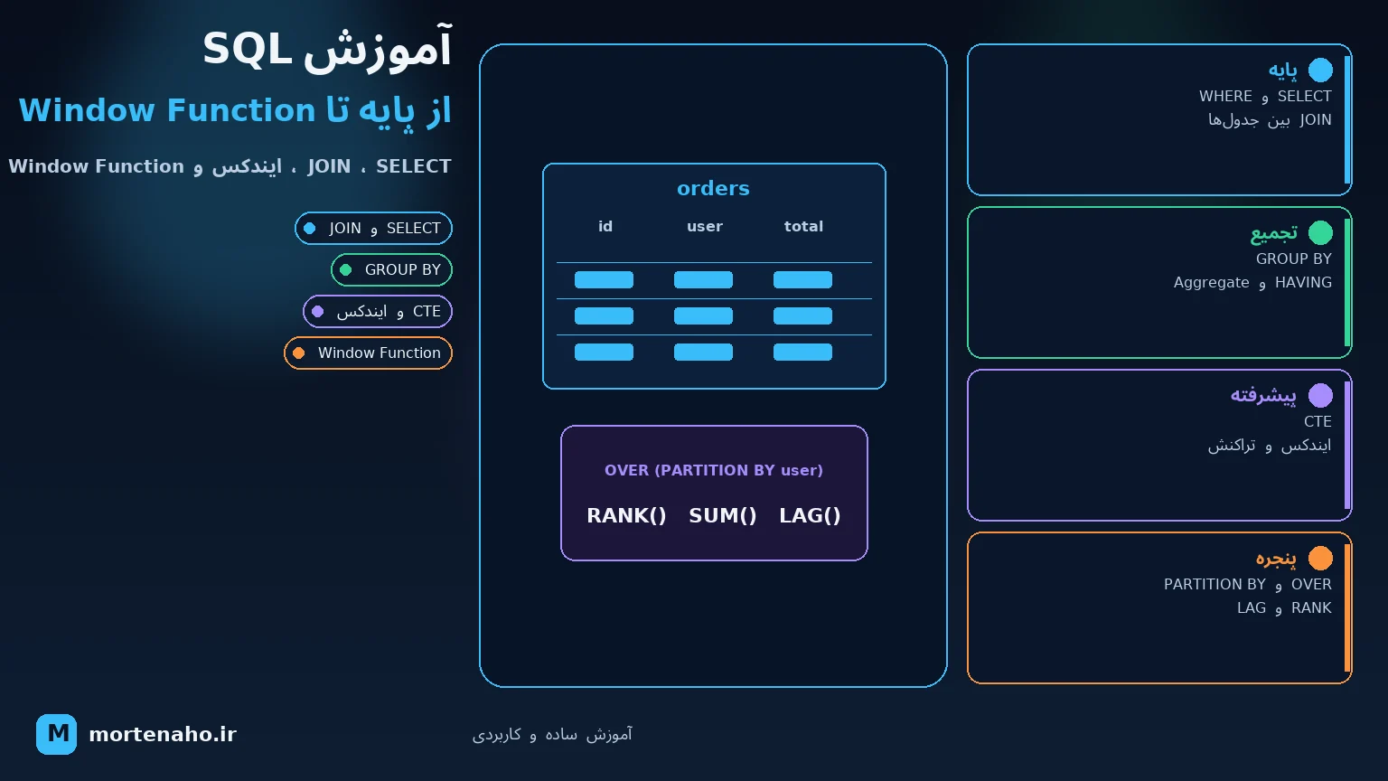
What you'll learn
This article is a complete SQL course — we start from zero and gradually move into professional topics. All examples use a simple shop database with four tables: customers, products, orders, and order_items, so you can apply the same logic in your own real projects.
Alongside basics like SELECT and JOIN, we cover Index, Transaction, and finally Window Functions — a powerful tool that many developers discover late.
1. What are SQL and a database?
A database is where an application's data is stored in an organized, persistent way — like customers, products, and orders in a shop. Unlike variables in application memory, database data survives when the program closes or even when the server restarts.
SQL stands for Structured Query Language — a language for talking to relational databases. With SQL you can define data (create tables), add or change data (INSERT, UPDATE, DELETE), and most importantly, read and filter data (SELECT).
Imagine storing a shop's information in separate Excel files: one for customers, one for products, and one for orders. As the shop grows, finding relationships between these files, preventing duplicate data, and ensuring data correctness quickly becomes hard. A relational database solves this by defining related tables and data integrity rules.
2. Types of databases and how they differ
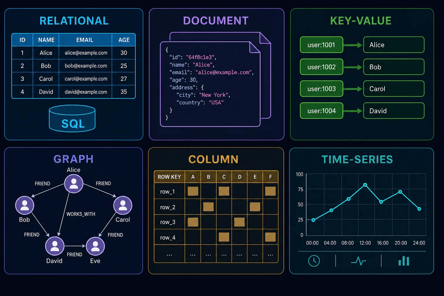
When we say "database," we don't mean only relational databases. Different models exist for storing data, each optimized for a particular kind of problem:
- Relational (e.g. PostgreSQL, MySQL, SQL Server, Oracle, SQLite): data lives in tables with fixed columns, and relationships between tables are defined with foreign keys. Its main language is SQL.
- Document (e.g. MongoDB): each record is a JSON-like document, and its structure can differ between records. Good for variable or nested data.
- Key-Value (e.g. Redis): data is stored as key-value pairs in memory or on disk. Read and write speed is very high; mostly used for cache and sessions.
- Graph (e.g. Neo4j): data is modeled as nodes and relationships between nodes. Good for social networks, recommendation systems, and complex paths between entities.
- Column-family (e.g. Cassandra): data is stored in a distributed column-oriented way, designed for very high write volume at multi-server scale.
- Time-series (e.g. InfluxDB or TimescaleDB): for data recorded with a timestamp, like sensor metrics and logs, where queries usually run over time ranges and aggregates.
| Database type | Examples | Data model | Best for |
|---|---|---|---|
| Relational | PostgreSQL, MySQL, SQL Server | Table with fixed schema | Transactional data, complex relationships, data integrity requirements |
| Document | MongoDB | JSON document with variable schema | Nested content, evolving data structure |
| Key-Value | Redis | Key and value | Cache, session, rate limiting |
| Graph | Neo4j | Node and relationship | Social network, fraud detection, product recommendations |
| Column-family | Cassandra | Distributed columns | Very high write volume, horizontal scale across data centers |
| Time-series | InfluxDB, TimescaleDB | Value with timestamp | Metrics, logs, sensor data, monitoring |
3. Basic relational concepts
Before writing your first query, let's learn a few basic terms:
- Table: a collection of same-type data with a fixed structure — like the
productstable for storing products. - Row: one specific record inside a table — for example one product with all its attributes.
- Column: one attribute of a record with a defined data type — like
price, which is always a number. - Primary Key (PK): a column or set of columns that uniquely identifies each row. Two rows cannot share the same PK.
- Foreign Key (FK): a column in one table that points to the primary key of another table and establishes a relationship — for example
customer_idin theorderstable referencescustomers. - NULL: means no value — not zero and not an empty string. If a customer's phone number was not recorded, that column's value is NULL.
4. Sample shop schema
In this tutorial we use a simple shop database: customers place orders, and each order includes one or more line items from the products table.
CREATE TABLE customers (
    customer_id   INT PRIMARY KEY,
    full_name     VARCHAR(100) NOT NULL,
    email         VARCHAR(150) NOT NULL UNIQUE,
    city          VARCHAR(80),
    created_at    DATE NOT NULL
);

CREATE TABLE products (
    product_id    INT PRIMARY KEY,
    product_name  VARCHAR(120) NOT NULL,
    category      VARCHAR(60),
    price          DECIMAL(10,2) NOT NULL,
    stock_qty     INT NOT NULL DEFAULT 0
);

CREATE TABLE orders (
    order_id      INT PRIMARY KEY,
    customer_id   INT NOT NULL,
    order_date    DATE NOT NULL,
    status        VARCHAR(20) NOT NULL DEFAULT 'pending',
    is_deleted    INT NOT NULL DEFAULT 0,
    FOREIGN KEY (customer_id) REFERENCES customers(customer_id)
);

CREATE TABLE order_items (
    order_item_id INT PRIMARY KEY,
    order_id      INT NOT NULL,
    product_id    INT NOT NULL,
    quantity      INT NOT NULL,
    unit_price    DECIMAL(10,2) NOT NULL,
    FOREIGN KEY (order_id) REFERENCES orders(order_id),
    FOREIGN KEY (product_id) REFERENCES products(product_id)
);
This schema is intentionally simple and portable across engines. For auto-incrementing identifiers, each dialect has its own syntax:
- PostgreSQL:
customer_id SERIAL PRIMARY KEYorGENERATED ALWAYS AS IDENTITY - MySQL:
customer_id INT AUTO_INCREMENT PRIMARY KEY - SQL Server:
customer_id INT IDENTITY(1,1) PRIMARY KEY - SQLite:
customer_id INTEGER PRIMARY KEY AUTOINCREMENT - Oracle:
customer_id NUMBER GENERATED ALWAYS AS IDENTITY PRIMARY KEY
5. Basic SELECT, WHERE, ORDER BY, and paging
The simplest query reads all columns or a few specific ones:
SELECT * FROM products;

SELECT product_name, price
FROM products;SELECT * in real code. List the columns you need explicitly so the query is faster and your application does not break unexpectedly when the schema changes.
Filtering with WHERE
SELECT product_name, price, category
FROM products
WHERE category = 'Electronics' AND price > 100;

SELECT * FROM orders
WHERE status IN ('pending', 'processing');

SELECT * FROM customers
WHERE city LIKE 'Tehran%';
Sorting with ORDER BY
SELECT product_name, price
FROM products
ORDER BY price DESC;

SELECT product_name, price
FROM products
ORDER BY category ASC, price DESC;
Removing duplicates with DISTINCT
SELECT DISTINCT category
FROM products;
Paging: LIMIT/OFFSET vs TOP and OFFSET-FETCH
When you only want some rows or one page of results, each dialect has its own syntax:
-- PostgreSQL, MySQL, SQLite
SELECT product_name, price
FROM products
ORDER BY price DESC
LIMIT 5 OFFSET 10;

-- SQL Server: simple version with TOP
SELECT TOP 5 product_name, price
FROM products
ORDER BY price DESC;

-- SQL Server: standard pagination with OFFSET/FETCH
SELECT product_name, price
FROM products
ORDER BY price DESC
OFFSET 10 ROWS FETCH NEXT 5 ROWS ONLY;
TOP without ORDER BY has no defined meaning; always specify a sort before TOP, LIMIT, or OFFSET/FETCH, otherwise results can differ between runs.
6. INSERT, UPDATE, and DELETE
Adding data with INSERT
INSERT INTO customers (customer_id, full_name, email, city, created_at)
VALUES (1, 'Sara Ahmadi', 'sara@example.com', 'Tehran', '2026-01-15');

INSERT INTO products (product_id, product_name, category, price, stock_qty)
VALUES (101, 'Wireless Mouse', 'Electronics', 249000, 40);
Updating data with UPDATE
UPDATE products
SET stock_qty = stock_qty - 1
WHERE product_id = 101;

UPDATE orders
SET status = 'shipped'
WHERE order_id = 5001;
Deleting data with DELETE
DELETE FROM order_items
WHERE order_item_id = 9001;
UPDATE and DELETE without WHERE run on every row in the table. Before pressing Enter, read the WHERE condition again, and if your tool allows it, first run a SELECT with the same condition to see the target rows.
Soft delete trick
Instead of physically deleting an order, it is usually better to mark it so it can be recovered and is not lost from historical reports:
UPDATE orders
SET is_deleted = 1
WHERE order_id = 5001;

-- Then add this condition to all normal queries
SELECT * FROM orders
WHERE is_deleted = 0;deleted_at TIMESTAMP NULL; if NULL the row is active, if it has a value the row was deleted and when.
7. JOIN between tables
JOIN combines two or more tables side by side based on a shared column (usually PK and FK). We look at the four main types with examples.
INNER JOIN — only rows that match on both sides
SELECT o.order_id, c.full_name, o.order_date
FROM orders o
INNER JOIN customers c ON o.customer_id = c.customer_id;
If a customer has no orders, they won't appear in an INNER JOIN result; only orders with a valid customer are returned.
LEFT JOIN — all rows from the left table, even without a match
SELECT c.full_name, o.order_id, o.order_date
FROM customers c
LEFT JOIN orders o ON c.customer_id = o.customer_id;
This query returns all customers — even those who haven't placed an order yet. For such customers, order_id and order_date will be NULL.
RIGHT JOIN — all rows from the right table, even without a match
SELECT c.full_name, o.order_id
FROM orders o
RIGHT JOIN customers c ON o.customer_id = c.customer_id;
This query returns exactly the same result as the LEFT JOIN example above — only the two tables are swapped in the query. RIGHT JOIN is used less often because the same logic can usually be written with LEFT JOIN and a different table order.
FULL JOIN — all rows from both sides
SELECT c.full_name, o.order_id
FROM customers c
FULL JOIN orders o ON c.customer_id = c.customer_id;
FULL JOIN (or FULL OUTER JOIN) shows both customers without orders and orders without a valid customer (if such inconsistent data exists).
FULL OUTER JOIN; you must build the same result with a UNION of a LEFT JOIN and a RIGHT JOIN. Older SQLite versions also lacked RIGHT JOIN and FULL JOIN; newer versions added both.
8. Aggregate functions, GROUP BY, and HAVING
Aggregate functions compute one value over many rows: COUNT, SUM, AVG, MIN, and MAX.
SELECT COUNT(*) AS total_orders FROM orders;

SELECT SUM(quantity * unit_price) AS total_revenue
FROM order_items;

SELECT AVG(price) AS avg_price, MIN(price) AS min_price, MAX(price) AS max_price
FROM products;
Grouping with GROUP BY
To compute aggregates per group, use GROUP BY:
SELECT p.category, SUM(oi.quantity * oi.unit_price) AS category_revenue
FROM order_items oi
JOIN products p ON oi.product_id = p.product_id
GROUP BY p.category
ORDER BY category_revenue DESC;
This query sums sales revenue per product category; the result has one row per category — far fewer rows than the total in order_items.
Filtering groups with HAVING
SELECT customer_id, COUNT(*) AS orders_count
FROM orders
GROUP BY customer_id
HAVING COUNT(*) > 2;
WHERE filters raw rows before grouping; HAVING filters after GROUP BY on each group's aggregate result. That is why you cannot use COUNT(*) directly in WHERE.
9. Subquery and CTE
Sometimes answering one query requires using the result of another query inside it:
-- Subquery in WHERE: customers who have orders
SELECT full_name
FROM customers
WHERE customer_id IN (SELECT DISTINCT customer_id FROM orders);

-- Correlated subquery: order count per customer
SELECT c.full_name,
       (SELECT COUNT(*) FROM orders o WHERE o.customer_id = c.customer_id) AS orders_count
FROM customers c;
When subqueries become nested and complex, a CTE (Common Table Expression) with WITH improves readability:
WITH customer_totals AS (
    SELECT o.customer_id, SUM(oi.quantity * oi.unit_price) AS total_spent
    FROM orders o
    JOIN order_items oi ON oi.order_id = o.order_id
    GROUP BY o.customer_id
)
SELECT c.full_name, ct.total_spent
FROM customer_totals ct
JOIN customers c ON c.customer_id = ct.customer_id
WHERE ct.total_spent > (SELECT AVG(total_spent) FROM customer_totals)
ORDER BY ct.total_spent DESC;
This query shows customers whose total spending is above the average spending of all customers. A CTE lets you name an intermediate result and reuse it in the main query without repeating the same logic.
10. Index and why it matters
An Index is like a book's table of contents; instead of reading the whole book to find a topic, the index takes you straight to the right page. In a database, an index is built on one or more columns and speeds up search, JOIN, and sort on those columns.
CREATE INDEX idx_orders_customer_id ON orders(customer_id);
CREATE INDEX idx_order_items_order_id ON order_items(order_id);
CREATE UNIQUE INDEX idx_customers_email ON customers(email);
Without a suitable index, the database must scan the entire table row by row (Full Table Scan) for each query — on a table with millions of rows that can be very slow.
WHERE, JOIN, or ORDER BY.
INSERT/UPDATE/DELETE must update indexes too. Indexing every column without studying actual query patterns (over-indexing) can slow writes down.
11. Transaction and ACID
A Transaction is a set of SQL statements that must all succeed or all be rolled back together — not half done. The classic example is placing an order while reducing warehouse stock:
BEGIN TRANSACTION;

UPDATE products
SET stock_qty = stock_qty - 1
WHERE product_id = 101 AND stock_qty >= 1;

INSERT INTO orders (order_id, customer_id, order_date, status)
VALUES (5002, 1, '2026-07-20', 'pending');

INSERT INTO order_items (order_item_id, order_id, product_id, quantity, unit_price)
VALUES (9002, 5002, 101, 1, 249000);

COMMIT;
If an error occurs midway — for example insufficient stock — use ROLLBACK to undo all changes in that transaction so stock and orders stay consistent:
ROLLBACK;The four ACID properties are the main reason to trust transactions:
- Atomicity: all statements in a transaction run together or none of them run.
- Consistency: after a transaction the database must remain in a valid state that follows its rules (like foreign keys).
- Isolation: concurrent transactions should not unintentionally affect each other's results.
- Durability: after a successful
COMMIT, changes survive even if the server shuts down unexpectedly.
12. Professional Window Functions
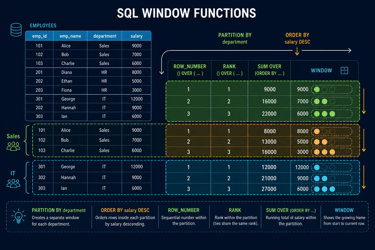
Unlike GROUP BY, which merges rows into groups and reduces the number of result rows, a Window Function computes a value for each row while keeping all original rows. Its main keyword is OVER().
PARTITION BY and ORDER BY inside OVER
PARTITION BY defines which group the calculation runs in (similar to GROUP BY, but without merging rows), and ORDER BY inside OVER sets the calculation order within that group.
ROW_NUMBER, RANK, and DENSE_RANK
SELECT c.city, c.full_name, ct.total_spent,
       ROW_NUMBER() OVER (PARTITION BY c.city ORDER BY ct.total_spent DESC) AS row_num,
       RANK()       OVER (PARTITION BY c.city ORDER BY ct.total_spent DESC) AS rnk,
       DENSE_RANK() OVER (PARTITION BY c.city ORDER BY ct.total_spent DESC) AS dense_rnk
FROM customers c
JOIN (
    SELECT o.customer_id, SUM(oi.quantity * oi.unit_price) AS total_spent
    FROM orders o
    JOIN order_items oi ON oi.order_id = o.order_id
    GROUP BY o.customer_id
) ct ON ct.customer_id = c.customer_id;
This query ranks customers by purchase amount within each city. The three functions differ in how they handle ties: ROW_NUMBER always gives a unique consecutive number; RANK gives the same rank to tied rows but leaves a gap in the next number; DENSE_RANK also gives the same rank but without a gap in the next number.
LAG and LEAD — compare with previous and next row
SELECT customer_id, order_id, order_date,
       LAG(order_date)  OVER (PARTITION BY customer_id ORDER BY order_date) AS previous_order_date,
       LEAD(order_date) OVER (PARTITION BY customer_id ORDER BY order_date) AS next_order_date
FROM orders;
LAG returns the previous row's value and LEAD the next row's value in the same partition — very useful for calculating the gap between two consecutive purchases by one customer.
SUM and AVG as Window Functions — running total
SELECT order_id, order_date,
       SUM(total_amount) OVER (ORDER BY order_date) AS running_total,
       AVG(total_amount) OVER (ORDER BY order_date ROWS BETWEEN 2 PRECEDING AND CURRENT ROW) AS moving_avg_3
FROM (
    SELECT o.order_id, o.order_date, SUM(oi.quantity * oi.unit_price) AS total_amount
    FROM orders o
    JOIN order_items oi ON oi.order_id = o.order_id
    GROUP BY o.order_id, o.order_date
) order_totals;
The running_total column shows cumulative sales up to each order, and moving_avg_3 computes a three-order moving average — both without losing the original report rows.
GROUP BY vs Window Function
| Feature | GROUP BY | Window Function |
|---|---|---|
| Number of result rows | One row per group | Same as input rows |
| Access to original row columns | Limited — only grouped or aggregate columns | Full — any original column can be selected |
| Compare with other rows in the same group | No | Yes — with LAG, LEAD, RANK, and similar |
| Good example | Total sales per product category | Rank customers in each city without losing each customer's details |
GROUP BY is enough. If you want to keep all original rows and add a group-related calculation beside each one, Window Functions are the right choice.
13. Important tips and common mistakes
- SQL Injection: never concatenate user input directly into an SQL string. Always use parameterized queries or prepared statements so input is treated as data, not as part of the SQL command.
- SELECT * in production code: transfers extra data, breaks code when the schema changes, and slows queries; select only the columns you need.
- UPDATE/DELETE without WHERE: without a condition, the command runs on every row in the table. Before executing, check target rows with a similar
SELECT. - Comparing with NULL:
column = NULLis always Unknown, not true. UseIS NULLorIS NOT NULLto test for NULL. - N+1 problem: running one query to get a list and then a separate query for each row (e.g. fetching each order's details with an independent query inside a loop) explodes database round trips. Instead, fetch everything you need in one JOIN or one batch query.
14. Short differences between dialects
| Topic | PostgreSQL | MySQL | SQL Server | SQLite | Oracle |
|---|---|---|---|---|---|
| Auto Increment | SERIAL / IDENTITY | AUTO_INCREMENT | IDENTITY(1,1) | AUTOINCREMENT | IDENTITY / Sequence |
| Paging | LIMIT/OFFSET | LIMIT/OFFSET | TOP or OFFSET/FETCH | LIMIT/OFFSET | FETCH FIRST n ROWS ONLY |
| Current date/time | CURRENT_DATE | CURDATE() | GETDATE() | date('now') | SYSDATE |
| Native Boolean type | Yes (BOOLEAN) | No; usually TINYINT(1) | No; usually BIT | No; 0 or 1 | No; usually NUMBER(1) |
| FULL OUTER JOIN | Yes | No (simulated with UNION) | Yes | Yes in newer versions | Yes |
15. Summary and checklist
- SQL is the language for working with relational databases; when choosing a database type, consider your data model and query patterns.
- Table, row, column, Primary Key, and Foreign Key are the foundation of every relational schema.
- With SELECT, WHERE, ORDER BY, and JOIN you can build most everyday reports.
- GROUP BY is for summarizing; Window Functions are for computing alongside original rows.
- Indexes speed up reads but are not free; add them only where needed.
- Put multi-step operations that must succeed or fail together in one transaction.
- Always parameterize user input and double-check the WHERE clause before UPDATE/DELETE.
The best way to learn SQL is to write queries on real data; build this shop schema in your database of choice and rerun the examples from this tutorial.